What percentage of “random fractions” have an even denominator? My friend Pig told me that the answer is around 1/3. (At least the answer is 1/3 for two somewhat natural definitions of the term “random fraction”.) Here is the experimental “proof” in Mathematica. ![]()
Mathematica input for test #1:
percentage[v_List, pred_] := N[ Length[Select[v, pred]] / Length[v] ];

percentage[ Table[ RandomInteger[{1, 1000}] / RandomInteger[{1, 1000}],
 {100000} ], EvenQ[Denominator[#]] ]
Output for test #1:
0.33343
Mathematica input for test #2:
percentage[ Table[i/j, {i, 1000}, {j, 1000}] // Flatten // Union,
            EvenQ[Denominator[#]] ]
Output for test #2 :
0.333443
Adam posted this code:

Related Posts via Categories
-
I have a quasiproof in the case where we consider fractions m/n with m,n bounded by N.
Let U_N be the rationals with numerator and denominator less than N. T_N those with numerator odd and S_N those with numerator even. Its clear that doubling N multiplies the sizes of these by 4. Now S_N is inside T_N. Multiplying members of T_N by 1/2 gives about half the members of S_2N, namely only those with denominators less than N. Thus 1/4 |T_N| = 1/2 |S_2N| so S is half the size of T. To finish the proof is easy now. Let m/n be a fraction with n even. Then n/m is a fraction with n even. So S is the same as T’. Thus T + T’ has size 3S.
-
Oops. There is a misprint. I meant S_N those with denominator even.
-
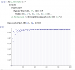
f[n_Integer] :=
Count[Flatten@(Apply[Divide, #, {2}] &@
Table[{x, y}, {x, n}, {y, n}]),
x_Rational /; EvenQ[Denominator[x]]]/n^2DiscretePlot[f[n], {n, 100}]
-
Adam, I tried to post an image generated by your code. It kinda worked.
-
Vance, I was thinking along similar lines, but my proof only worked for random fractions R = I/J where I and J were random integers over a finite range.
-
Suppose I want an analytic expression for a probability measure on the set of rationals in (0,1) such that the probability of a fraction having an even denominator is exactly 1/3.
1. Is this easy?
2. What about the same question for numerator instead of denominator? (ha ha, sigh….)
-
Well, I have a suggestion. Suppose S is a set of rationals in (0,1). Let U_N be the set of rationals m/n in (0,1) with m<n=<N. Let S_N = U_N intersect S. Then define the measure of S to be the limit |S_N|/|U_N| assuming this limit exists.
-
I think, under Vance’s definition, that the “measure of S” would be 1/3 if S was the even denominator rationals, but I might be too lazy to try to prove it. – Hein
-
antianticamper, the rationals m/n between 0 and 1 are the reciprocal of the rationals bigger than 1, so I imagine 1/3 of the rationals between 0 and 1 have even numerators.
-
Chris Commented:
I fixed that problem, maybe I just sent it to Carl. Maple’s random number generator for rational’s is not working the way I would expect it to work. I’ll send them a note, since it’s used as an example in their documentation.
OK, not to belabor the whole thread, but this whole question has bothered me, not in the statement, which is clear, but in the empirical demonstration. Let me explain:
Prop: The probability of choosing a (reduced) rational with an odd denominator is 2/3.
Proof: Reduced rationals have the form O/E, O/O or E/O (E/E is not possible) so 2/3 times at random you pick a rational with an odd denominator. Check!But you’re experiment shows that if you pick two integers at random and compute their reduced fraction you also get an even denominator 1/3 of the time — which makes sense, until you think about the following experiment: suppose I am going to choose two integers at random, divide the first by the second and reduce the fraction. Before going to the “experiment” part, remember by the fundamental theorem of arithmetic (FTA):
O = $3^p 5^q 7^r\ldots$ while
E = $2^n 3^p 5^q 7^r\ldots .$Where for E, n >= 1. Now, the outcomes of my experiment are:
Case 1: O followed by O, which always reduces to O/O, (as you can see by the FTA). Event Probability = 1/4
Case 2: E followed by O, which always reduces to E/O, (as you can see by the FTA). Event Probability = 1/4
Case 3: O followed by E, which ways reduces to O/E, (as you can see by the FTA). Event Probability = 1/4
Case 4: E followed by E, which now has two possibilities (but a gross event probability of 1/4):
Say that $E_1 =2^n r_1$ (where $r_1$ is the extra prime power multipliers) and
$E_2 = 2^m r_2$ (where $r_2$ is defined analogously)Case 4.1: If $n >= m$ then the fraction reduces to E/O or O/O so you get an odd number denominator
Case 4.2: If $n < m$ then the fraction reduces to O/E, with an even number denominator.Here comes the weird part. Let’s say that I want to know the probability that this E/E works out to have an odd denominator. I apply my first proposition and I get this neat formula which is:
Probability of odd denominator = 1/4 + 1/4 + (1/4 * 2/3) = 2/3
Probability of even denominator = 1/4 + (1/4 * 1/3) = 1/3.So this validates the result BUT WAIT! Let’s look back at the FTA. We’re really asking something about m and n above, right? We’re saying we’re choosing two random integers (both happen to be even) and then with that as our conditioning statement, we’re saying what’s the probability that $m\geq n$ (vs. $m < n$). Doesn’t that feel like it should be 1/2 (as you let m and n go to infinity to scoop up all the integers?) What the hell is happening here?
This may be a lot of rambling and I could be tired from my plane ride, but something funny is being illustrated by this experiment in terms of the FTA viz. random choice of integers and I’d like to know if I’m crazy or stupid or if there’s really something deeper here.
-
At first it would appear that $P(n \geq m)$ would be approximately equal to $P(n < m)$; however, I am pretty sure that our intuition is wrong here. In fact, I think that
$$P(n > m) \approx P(n < m) \approx P(n = m).$$
Technical Notes: If $I$ and $J$ are random integers from the set $\{ 1, \dots, 2^k \}$ and $M = \max \{\, j : 2^j | I \,\}$ and $N = \max \{\, j : 2^j | J \,\}$, then I think $P(N = M) \approx P(N > M) \approx P(N < M)$.-
That’s an interesting “technical note.” It reminds me of a paper I was reading back when I was a “big data” guy (last month).
http://metamarkets.com/2012/fast-cheap-and-98-right-cardinality-estimation-for-big-data/
-
I just noticed something in the wikipedia article on the zeta function. If two integers are chosen at random, then the probability that they are coprime is 1/zeta(2). So it looks like if you want to do numerical experiments on sets of rationals using a random number generator, you can just generate pairs of random integers and throw out a pair if is not coprime.
-
The $Pr(n m)$ doesn’t seem to be right in experiment. Here’s my Maple output:
pCount := 0;
qCount := 0;
N := 100000;
for i to N do
v := Generate(integer(range = 0 .. 10000));
u := Generate(integer(range = 0 .. 10000));
if v > u then
pCount := pCount+1
else
qCount := qCount+1
end if
end do;
unassign(‘i’, ‘v’, ‘u’);evalf(qCount/N);
0.4983500000
evalf(pCount/N);
0.5016500000Maybe I’m missing something deeper that everyone else is saying.
-
Integers have two natural structures: additive and multiplicative. Each structure is relatively simple by itself, but the interplay between them can be quite deep and complicated. And sometimes the distinction is just easy to overlook.
For example, each structure has it’s own natural “absolute values”. The natural absolute value for the integers considered as an additive group is the standard Archimedean absolute value: $|x| = x$ if $x \ge 0$ and $|x| = -x$ if $x < 0$. There are many natural absolute values for the integers considered as a multiplicative group, however: $|x|_p = 1/p^{v_p(x)}$ for each prime number $p$, where $v_p(x)$ is the highest power of $p$ that divides $x$. ($v_3(9) = 2$ and $v_7(1/49) = -2$, for example.)
Before I continue, a few comments. First, the absolute values $|\cdot|_p$ are called "non-Archimedean" because they satisfy a stronger triangle inequality: $|x + y|_p \le \max(|x|_p, |y|_p)$. Second, the standard Archimedean absolute value is sometimes called the "absolute value at infinity" and denoted $|\cdot|_\infty$. Finally, with these conventions we have the identity (for any rational $x$):
$$\prod_p |x|_p = 1$$
where the product is over all "finite primes" and the "prime at infinity". Number theorists sometimes joke that real analysis is "number theory at infinity!"Now, consider the harmonic series
$$\sum_{n \ge 1} {1 \over n} = 1 + {1 \over 2} + {1 \over 3} + \ldots$$
and the identity
$${1 \over 1 - x} = 1 + x + x^2 + \ldots$$
Setting $x = 1/p$ this identity becomes
$${1 \over 1 - 1/p} = 1 + {1 \over p} + {1 \over p^2} + \ldots$$
and then by the Fundamental Theorem of Arithmetic we have
$$\sum_{n \ge 1} {1 \over n} = \prod_{p {\text { prime}}} {1 \over 1 - 1/p}$$
as formal expressions.To make the expressions converge we can do one of two things. First, we can add an exponent to the denominators, in which case we have
$$\sum_{n \ge 1} {1 \over n^s} = \prod_{p {\text { prime}}} {1 \over 1 - 1/p^s}$$
and both sides converge and are analytic for $\Re s > 1$. This, of course, is the Riemann zeta function $\zeta(s)$, and the product on the right-hand side is why it’s important.The other way to make the expressions converge is to limit the number of terms (or factors):
$$\sum_{n < N} {1 \over n}$$
and
$$\prod_{p < N} {1 \over 1 – 1/p}$$It is easy to see that $\sum_{n < N} {1 \over n} \sim \log N$; what about $\prod_{p < N} {1 \over 1 – 1/p}$? Obviously the two expressions aren’t equal, but do we have
$$\sum_{n < N} {1 \over n} \sim \prod_{p < N} {1 \over 1 – 1/p}$$
as $N \to \infty$? The answer turns out to be ‘no’ (although they are of the same order as $N \to \infty$), but the point I’m trying to get to is that the sum is limiting the size of the denominators of the fractions additively, while the product is limiting the size of the denominators (in the multiplied-out sum) multiplicatively, and therefore different fractions are included in each sum.In essence, we have defined two different measures to measure the size of fractions. And likewise two different distributions for “random” fractions.
Now the punch line: given the first distribution, fractions with even denominators show up $1/3$ of the time; given the second, even denominators show up $1/2$ the time. But since both distributions are natural, and since they are similar to each other, it is easy to miss that they are actually different!
-
I’ve tested a mixture of Hein’s conjecture with my argument to show that while Hein’s idea that Pr(n=m) = Pr(n > m) = Pr(n m) = Pr(n < m) = 1/3. Obviously to be precise, everything is assuming a discrete uniform distribution. This is illustrated in my little Maple experiment.
To prove this statement, I suspect we require Carl's insights. I'd also note, there is something interesting and counter-intuitive happening here viz. the uniform distribution over the integers.
What seems to be interesting is that the factorization is twisting the uniform distribution in a cute way [in response to Vance's comment by e-mail that looking at the prime factorization causes us to look at an entirely different distribution.
OK, here's the little experiment in Maple:
with(RandomTools);
TwoPower := proc (N::integer)::integer;
local M, count;
M := N; count := 0;
while modp(M, 2) = 0 do
count := count+1;
M := (1/2)*M
end do;
count end proc;Simulate := proc (N::integer)::list;
local eCount, oCount, nlCount, nhCount, neCount, tpn, tpd, i, num, deno, fra, dd;
eCount := 0;
oCount := 0;
nlCount := 0;
nhCount := 0;
neCount := 0;
for i to N do
num := RandomTools:-Generate(integer);
deno := RandomTools:-Generate(integer);
fra := num/deno; dd := denom(fra);
if modp(dd, 2) = 0 then
eCount := eCount+1
else oCount := oCount+1
end if;
tpn := TwoPower(num);
tpd := TwoPower(deno);
if tpn < tpd then
nlCount := nlCount+1
elif tpn = tpd then
neCount := neCount+1
else nhCount := nhCount+1
end if end do;
[eCount, oCount, nhCount, neCount, nlCount]
end proc;evalf((1/10000)*Simulate(10000));
[.3335000000, .6665000000, .3331000000, .3334000000, .3335000000]# The previous example illustrates that for the appropriate measures, fractions with
#even numerators show up 1/3 of the time and illustrates Hein's conjecture that 1/3 of the
#two integers are chosen with the 2's in their prime factorizations having equal powers.#
# Proving that will likely require the post Carl made.#In order of output, we have the proportion of times an even number is the denominator;
#the proportion of times an odd number is the denominator;
#the proportion of time the random integers have a higher power of two in the prime
# factorization on the (non-reduced) numerator; an equal power of two in the prime
# factorizations of the two integers and; a lower power of two in the prime factorization
# of the (non-reduced) denominator. -
So it seems that there is enough interest that I should write down a “proof” of my previous statement
If $I$ and $J$ are independent random integers from the set $\{ 1, \dots, 2^k \}$, $M$ is the largest integer such that $2^M$ divides $I$, and $N$ is the largest integer such that $2^N$ divides $J$, then
P(N is less than M), P(N equals M), and P(N is greater than M) are all about 1/3.
“Proof”
It is fairly obvious that P(N is less than M) = P(N is greater than M). So now we compute $P(N=M)$.
$P(N=M)$
$\ \ = \sum_{i=0}^k P(N = i \ and \ M= i) $
$\ \ = \sum_{i=0}^k P(N = i) P(M= i)$
$\ \ = \sum_{i=0}^k 2^{-i-1} 2^{-i-1}$
$\ \ = \sum_{i=0}^k 4^{-i-1}$
$\ \ = {{1/4- 1/4^{k+2}}\over{1 – 1/4}}$
$\ \ \approx {{1/4}\over{1 – 1/4}}$
$\ \ = 1/3.$
-
The crux of this argument is the value for P(N=i) in this logarithmic distribution. If we change the base to 3, say, then this value changes and we get a very different answer. Also, I am not sure how you arrived at the value you use.
I get something like Pr(N=i)=(2^i – 2^(i-1))/2^k = 2^(i-1-k). I think this does not change the answer because it reverses the order of the summands.-
Just to make sure I am understanding the notation correctly, we have
$$Pr(N = 0) = {1 \over 2},\quad Pr(N = 1) = {1 \over 4},\quad Pr(N = 2) = {1 \over 8},\quad\ldots$$
correct? In particular, the probability that a random integer is divisible by a higher power of a prime is less than the probability that it is divisible by a lower power of the same prime. Therefore I don’t think the formula
$$Pr(N = i) = (2^i – 2^{i – 1}) / 2^k = 2^{i – 1 – k}$$
is correct. I think the correct formula is
$$Pr(N = i) = {1 \over 2^{i + 1}}?$$-
Yes, I was wrong. I misread the definition. I thought we were asking for the probability that m was between 2^(i-1) and 2^i. Instead we are asking for the number of trailing zeroes in the binary representation. So the probability that the last bit is 1 is 1/2, the probability that the last bit is 0 and the next to the last bit is 1 is 1/4 and so on.
-
Hi Carl, I think your formula is almost perfect. In the situation where the numerator and denominator are between 1 and $2^k$, I think to be 100% correct you need to account for the edge cases as follows:
$$P(N=i) = {1\over{2^{i+1}}}$$
when $i$ is an integer with $0<= i < k$, $P(N=k) = 1/2^k$, and $P(N=i) = 0$ otherwise. I didn’t take care of the edge cases in my “proof” because I did not think it through carefully.
-
OK…I agree with Hein’s proof (now that I understood what he was actually saying). Though I can see Vance’s point. For instance, I get
Pr(N = i) = 1/2^{i}
but my sum goes from i = 1 to k, so it all boils down to the same thing. I think we’ve beaten this thing to death. It’s nice to know that this works and it’s all very cute.
-
-
-
-
-
-
Comments are now closed.
22 comments